Author's note: This article is based on Bell's Theorem (1). I have reformulated the presentation to make it a little easier to see that "Negative Probabilties" are a seemingly paradoxical consequence of his work. The Bell Inequalities can be presented in many forms, and most are essentially equivalent. I do not know if this particular presentation format or derivation has been used by others, I can only assume it has. I follow conventional interpretation of both QM (quantum mechanics) and Bell. I assume the reader already has basic familiarity with Bell test setups such as Aspect(2). For a more rigorous proof, look to Bell, Aspect and others.

Figure 1:
John S. Bell (1928-1990), author of Bell's Theorem. We don't need to see the pocket protector to know this guy is a major geek.
Some have posed the question, "How does Bell's Theorem lead to predictions of negative probabilies?" We will answer that here. Bell created his theorem in response to Einstein's last major paper (3), which is often called the EPR Paradox. EPR states that if Quantum Mechanics (QM) is complete (and there are no "hidden variables"), then there cannot be simultaneous reality to non-commuting operators. Einstein himself took this to mean that since there MUST be "simultaneous reality to non-commuting operators" (any other position was unreasonable, he maintained), then QM was NOT complete and therefore hidden variables existed.
(Hidden variables means that there are microscopic properties of fundamental particles that we are unable to observe directly by means of testing, perhaps due to technological limitations that might not exist at some future time. Since we can't observe them, they are "hidden" now - but perhaps if we knew more about them then that might explain the otherwise mysterious behavior of particle spin.)
Bell saw it differently. He took EPR at face value, as many physicists did, and concluded that there were no hidden variables. A strange position, to be sure, but not contradicted by the facts. Building from this position, he then went further: he showed that hidden variables would lead to a disagreement with the predictions of QM in certain specific cases (see Figure 2 below). Please recall: a single counter-example is sufficient to disprove any theory, and this forms the basis of our argument. So Bell's Theorem is based on EPR, and demonstrates that the following 3 things cannot all be true (i.e. at least one must be false):
i) The experimental predictions of Quantum Mechanics are correct with respect to spin predictions (a testable hypothesis)
ii) Hidden variables exist (particle attributes really exist independently of observation - this is akin to saying that the moon is there when you are not looking at it); and
iii) Locality holds (a measurement at one place does not affect a measurement result at another, more or less in accordance with Einstein's Special Theory of Relativity which makes the speed of light a universal "speed limit").
QM predicts that certain classical scenarios, if they existed, would have negative likelihood of occurance (in defiance of common sense). Any so-called local realistic theory - in which ii) and iii) above are assumed to be true - will make predictions for values of these scenarios which are significantly different than the QM predicted values. QM does not acknowledge the existence of these scenarios, often called hidden variables (HV), so it does not have a problem with this consequence of Bell's Theorem. (I.e. there are no negative probabilities in QM itself.) We will ignore the iii) case here, as if you accept that locality fails anyway then there is no particular conflict between i) and ii). In other words, we assume that Einstein's Special Relativity holds in the sense that causes cannot propagate to the future faster than c (the speed of light). Again, our objective is to see the effect of the "hidden variable" or "Realistic" assumption and how that specifically leads to results that defy our intuitive common sense.
In the entangled photon scenarios, the Realistic view - which maps to assumption ii) above - states that the photon polarization is determinate as of the point in time that the photons' existence begins. The attribute we measure is considered "determinate" because its value is determined *before* the act of measurement. To repeat, this is a questionable assumption as we shall see below. Even though the entangled photons can only be measured at 2 different angles before they are disturbed, the Realistic view states that they could potentially have been measured at other angles as well. Thus, the Realistic view is that the existence of the photon polarization is independent of the act of measurement (and is a result of the state of the hidden variables). On the other hand, QM (Heisenberg Uncertainty Principle) says that the photon spin (polarization) exists only in the context of a measurement, and the the act of observation is somehow fundamental to the measurement results. Here is the paradox that is a partial result of Bell's Theorem:
Proof
a. Let there be 2 single channel photon detectors with matching polarizers. I will call them Left and Right (see basic setup in the chart below). They will be positioned so that a beam of entangled photons (a la the Clauser/Horne/Shimony/Holt setups) will strike them sometime after they are created, a point in time which we shall call Time(created) or T=0. The beam then passes through the optical polarizers that then filter out half of the photons at a later time, leaving the other half to be detected. The later time is only a fraction of a second later, which for our purposes we will call Time(measured) or T=1. The key element is that measurement occurs after the entangled state is created:
Time(created) < Time(measured)
The requirement is that causes must precede their effects, because the act of measurement at one spot is not responsible for the results measured elsewhere (i.e. outside of an Einsteinian light cone). As stated in iii) above, we are not adhering to this strictly here. Essentially, we are assuming that it is correct so we can see what else happens in such a scenario. There are enough definitions of determinism, locality, causality, FTL, etc. that they form a separate discussion outside of our current scope of interest. If you believe that the future can influence the past, then you can explain away the negative probabilities we end up with below.
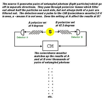
The Left is set at angle A=0 degrees. The Right is set at B=67.5 degrees. We will consider that there is the possibility that we could also measure the polarization at another angle in between the settings of Left and Right detectors, and this angle is for the sake of discussion called C=45 degrees. It does not matter for the purposes of this discussion whether we measure C on the Left or the Right, the only thing that matters is that we can conceptualize that such a measurement could have been made; i.e. the polarization exists independently of the act of observation. In each case, the angle settings are adjusted so that 0 degrees difference would mean that there is perfect correlation, as is true in both classical and quantum mechancial scenarios in the ideal case. A difference of 90 degrees means there is perfect anti-correlation, also identical in all scenarios. Our selection of the angles is not random, it is done specifically to highlight the desired conclusion. Let's call it + if there was a detection at that spot, and - if there is no detection. Practical detector efficiencies and actual experimental requirements are ignored.

Figure 2:
Basic diagram of a Bell test experiment with single channel polarizers; in single channel tests we refer to polarization as + or - with a + meaning the photon was detected. The polarizer angle can be varied and the test re-run. The + and - results from each side are compared and the correlations are counted. The correlation percentage is then computed. The +/- pattern is completely random for either detector. However, for entangled photon pairs, a pattern only emerges once the detector results are compared. Creating entangled pairs is very difficult, and requires special apparatus.
b. In the Realistic view, we could imagine that A, B and C all exist at the same time - even if we could only measure 2 at a time. In the words of Bell: "It follows that c is another unit vector [in addition to a and b] ...". Therefore, there are 8 possible outcomes that must total to 100% (probability=1). This is "common sense". The permutations are:
